Data Collection

Data Collection Overview

Addressing our problem statement entails understanding the sequence in which apps are launched and how much time is spent on each app. Additional features such as app window placement may indicate the likelihood of usage. To generate this data and required features, we built input libraries in C/C++, utilizing windows APIs from Intel’s proprietary XLSDK library. Each input library extracts data alongside collection timestamps. These input libraries are:

• mouse_input.IL
• user_wait.IL
• user_wait.IL
• desktop_mapper.IL

Mouse Input IL

The mouse_input.IL project served as a predicate to the other input libraries. This task was designed to help us familiarize ourselves with the Windows development environment and accompanying configurations. As such, we incorporated Intel provided code into the static_standard_library sample template. The goal of this IL is to store and predict mouse movement data. Every 100 ms, we track the x and y position in pixel(s) of the mouse cursor and apply a 1D Kalman predictor to expose the inputs. We track the mouse noise in both the x and y positions as well as the Kalman predicted value in both dimensions. The following tables are the outputs of the mouse_input.IL:

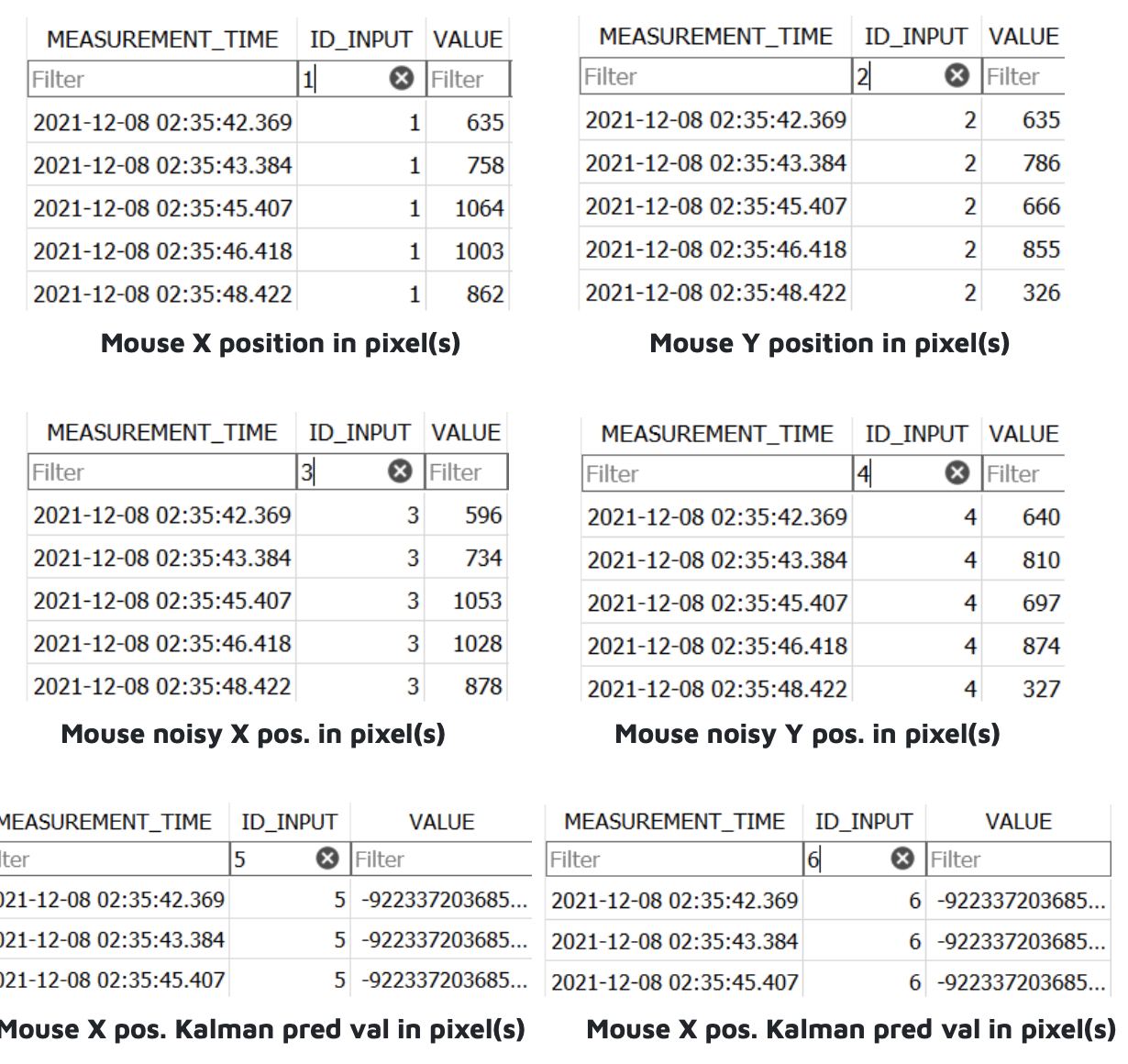
We faced a bug with the Kalman predictor wherein it only logged negative float values.

User Wait IL

The purpose of the user_wait_IL is to obtain the cursor type and accompanying usage times. We built this IL off the static_standard_pure_event_driven sample template. This project required the creation of a collector thread which monitors the state of the mouse cursor icon at regular intervals (every 100ms). We initialize an array of handles containing references to 16 different mouse cursors (ex. Standard arrow, arrow with spinning wheel, etc.). Our thread process calls the custom_event_listener_thread function, setting off an infinite while loop which runs until it receives the stop_request (when the user presses CTRL+C). Inside the loop, we implement the WaitForSingleObject API function which tracks timestamps in 100 ms pause intervals. During each pause, we store the size of the current mouse cursor and retrieve the current cursor handle using GetCursorInfo. We compare the current handle against every handle in our handle array and store the index of our array where the handles match. This way, we have mapped an integer value to the mouse cursor handles and saved storage space. As soon as the while loop is interrupted, we exit the thread and handle any possible errors.

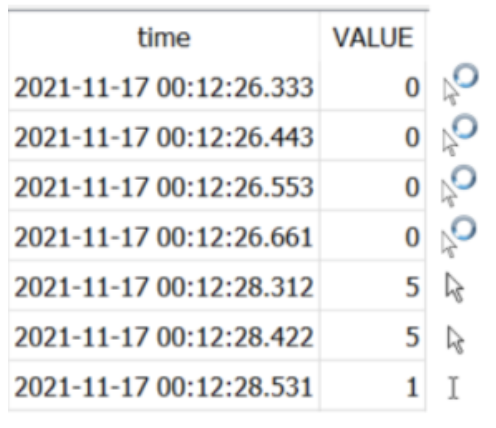
The outputs are automatically generated in a SQLITE database file. In the sample on the right, we see that the cursor value of 0(app starting) changes to 5 (standard arrow) and then to 0 (ibeam cursor) when we launch photoshop, then open MS Word and start typing.

Upon collecting and verifying this data, we performed data wrangling on the output tables. We narrowed our scope to only a few frequently appearing cursor types out of the 15 mapped icons in our data. These include the IDC_APPSTARTING, IDC_ARROW, IDC_HAND, IDC_IBEAM, and IDC_WAIT cursor icons. All other cursor types are classified as “OTHER”. We may wish to only examine app launch times using the IDC_APPSTARTING icon in which case our data will be engineered to contain binary inputs.
As this was our first time building an input library in C++ by ourselves, we struggled to navigate the MSDN and understand the windows API functions. However, with some help from Jamel, we were able to debug our issues, and collect data successfully.

Foreground Window IL

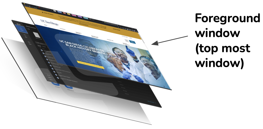
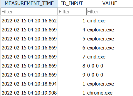
The purpose of the foreground_window IL is to detect and log the name of the executable whose app window sits atop all others. We implemented two waiting events to trigger the foreground window check: mouse clicks, and 1000ms time intervals.
To detect these two events, we created a collector thread which calls on the WaitForMultipleObjects api function. As in user wait, an infinite while loop runs until it receives the stop_request (CTRL+C). To limit the size of our output, we made the decision to log the foreground window only if it is different from the previous foreground window. Therefore, we check if the current window’s process ID is different from the previously stored process ID. If so, we retrieve the executable token (the string.exe name) of the new foreground window and log it to our output table. Additionally, we captured the features “isImmersive” which checks if a process belongs to a Windows store app and “isHung'' which checks if the foreground window is unresponsive. Upon each detected foreground window change, we emit a custom IDCTL signal with the message “FOREGROUND-WINDOW-CHANGED” to be processed by the desktop_mapper IL. The collector pauses if the device enters screen-saver mode or a mouse is clicked over the collector, and stops running when CTRL+C (stop signal) is clicked. The string outputs appeared as expected in the form of app executable names. The accompanying isImmersive and isHung binary features are located in a separate table.

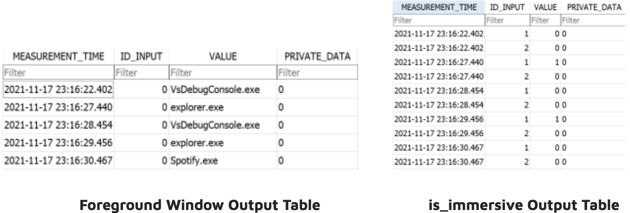
The primary challenge we faced in the foreground_window.IL was in regard to duplicate exe strings being logged with different timestamps despite our process checking logic. We deduced that this was because the user was using split windows for the app, resulting in two separate processes, and alternating their mouse back and forth between them. Since the split windows were for the same app executable, we decided to drop consecutive duplicates. This does not affect time spent on the app executable as this is calculated from the first measurement timestamp.

Desktop Mapper IL

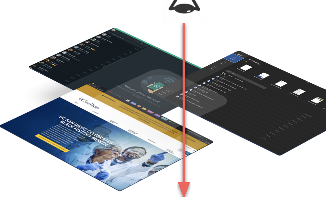
The Desktop Mapper input library was the most challenging to develop. The aim is to take a snapshot of the desktop and understand where app windows are located with respect to each other. Therefore, it functions by iterating through the z-axis of app windows, going from top to bottom, collecting data on each window’s properties. We collected each windows executable name, as well as that of the windows above and below it. We also collected information on the position and size of the window rectangle. To trigger Desktop Mapper data collection, we wait for a signal denoting a change in foreground window. This starts the collector thread, which stores all the window properties in a desktop array. After data collection is complete, the logger thread logs the desktop array to an output table. To ensure that no processes overwrite each other or the output table, we used best practices for thread safety. 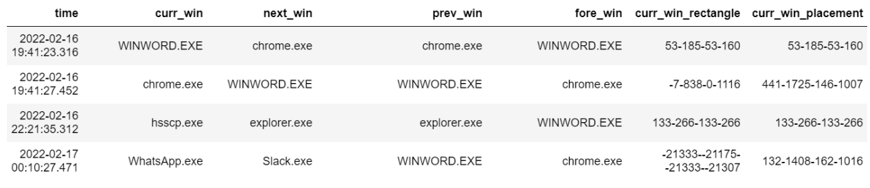The output table contains stacked values of features including:

• Current Window Executable Name
• Next Window Executable Name
• Foreground Window Executable Name
• Current Window Rectangle
• Current Window Placement

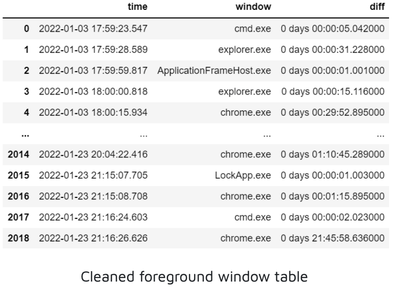
Other window features, is_visible, is_minimized, is_maximized, and is_hung were also collected, however, no valuable information was captured with these features. After some hefty data cleaning, we are able to map a relatively messy table into a relatively clean table.

The second problem is to predict app usage durations and corresponding app sequences.

Using a custom built python script, we are able to clean this messy table and turn it into a multi-column pandas dataframe.

Challenges

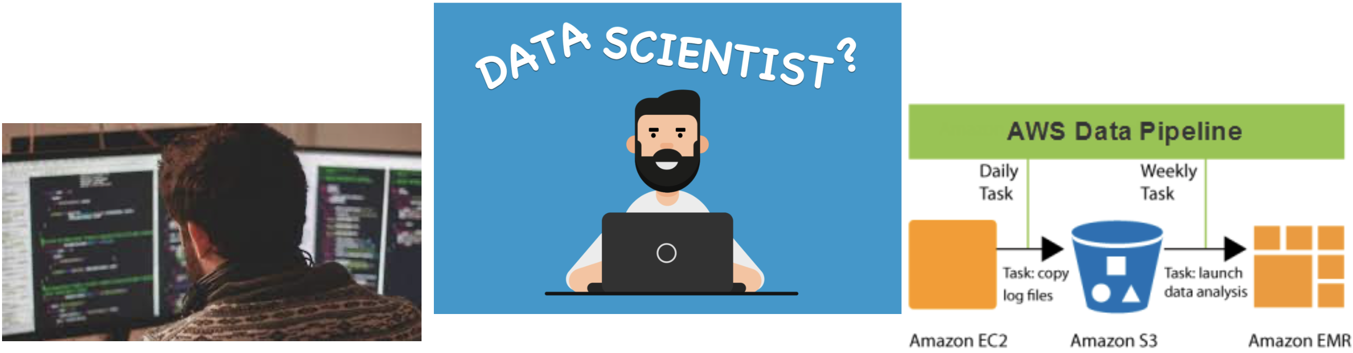
As conventional Data Scientists, our skill-sets prior to this project revolved around python and data modeling. Stepping into the shoes of a software engineer and using C for pushing production-ready code was challenging and posed a steep learning curve. In the foreground window, we noticed that duplicate executables were sporadically being outputted but with different timestamps. We deduced this was because the user had split tabs of that app open or they were changing the size of the windows. We handled this issue by dropping the consecutive duplicates since they account for the same executable. In the desktop mapper, we noticed that our collector had a shadow period between the data collection time and the logging time. Since we’re iterating through all desktop windows, it takes time to perform the data collection. And during that time, we might be changing between several foreground windows. This results in backed up logs with wrong timestamps, and a similar duplicate issue as we faced earlier. Fixing this will require us to spend a bit more time optimizing the collector.

EDA

Exploratory Data Analysis

For any data science problem we need good quality data and being able to control the process of collection allows us to build features for our prediction problem. Since we were not provided any historic data for this project, we spent 10 weeks building data collector modules. They capture cursor type, active foreground windows, and window placement data which allows us to better understand the app usage behaviour of our users. Our collectors run in a low state mode without taxing system resources, allowing the user to use their computer naturally. We ran these collector modules on our personal devices for 3 weeks while university was in session. We collected three weeks of data on two of our personal PCs starting from January 3rd. User1 had 32 unique apps while user2 had 25 during the data collection period. We noticed that most of the daily activity for both users revolved around chrome. In fact, chrome made up 30% and 35% of user1 and user2’s data, respectively. The second most common app, explorer.exe or the file explorer, made up around 18% and 20% of user1 and user2’s data, respectively. The remaining app windows constituted less than 10% each, meaning both datasets are heavily imbalanced. Below are a series of visualizations and corresponding insights:

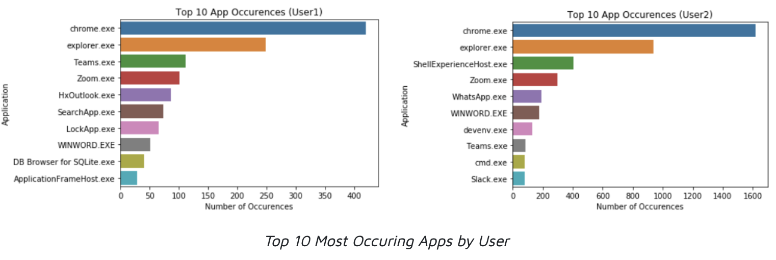
Insights: Most of the daily activity for both users revolved around chrome. Chrome made up 30% and 35% of user 1 and user 2’s data, respectively. The second most common app, explorer.exe or the file explorer, made up around 18% and 20% of user 1 and user 2’s data, respectively. The remaining app windows constituted less than 10% each. User 1 had a total of 32 unique apps while user 2 had 25.

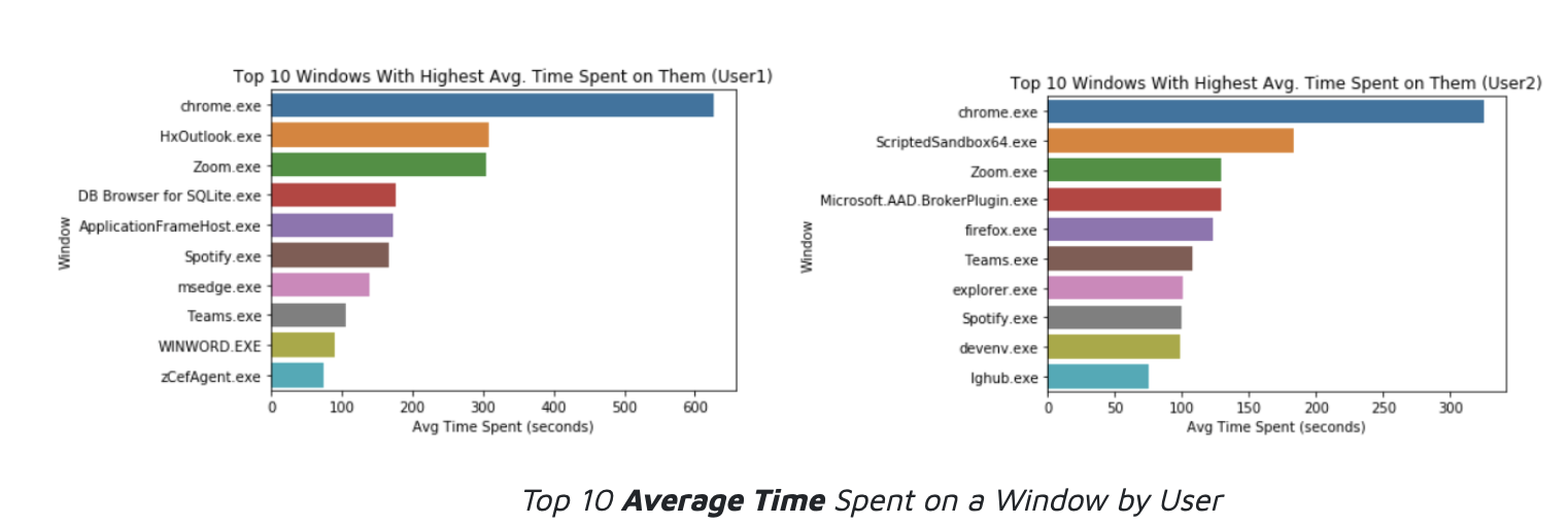
Insights: These plots represent the top 10 average amount of time (in seconds) spent on a window over the course of the data collection period for each user. Outliers of 9+ hours (>15,000 seconds) were eliminated since they represented idle times.

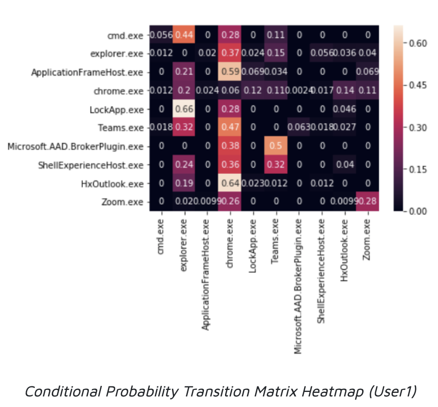
Insights: This heatmap represents the transition matrix for our HMM. The elements are the conditional probability of the column window appearing after the row window. The dark values represent low switching probabilities while lighter colors represent higher probabilities.

Prediction

Prediction Overview

Prediction Problem 1

We came up with 2 prediction problems to better understand app usage behaviors, using 3 weeks of our collected time-series window data starting from January 3rd 2022.
The first problem is to identify patterns in app launches.

The HMM is best suited for our first problem as it allows us to understand the progression of events based on conditional probabilities. It works on the assumption that the future state relies on the current state which is important considering we are using sequential window data. We implemented three predictors using different heuristics for measuring accuracy to see how they compared with each other.

Hidden Markov Model

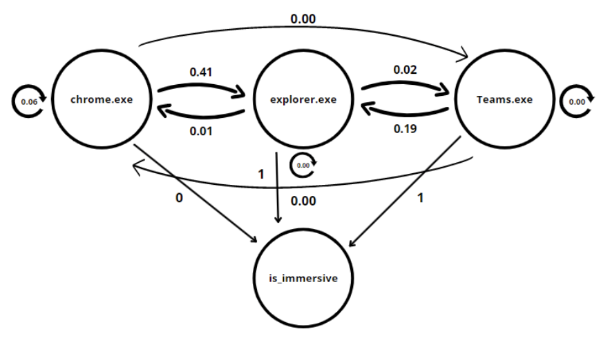
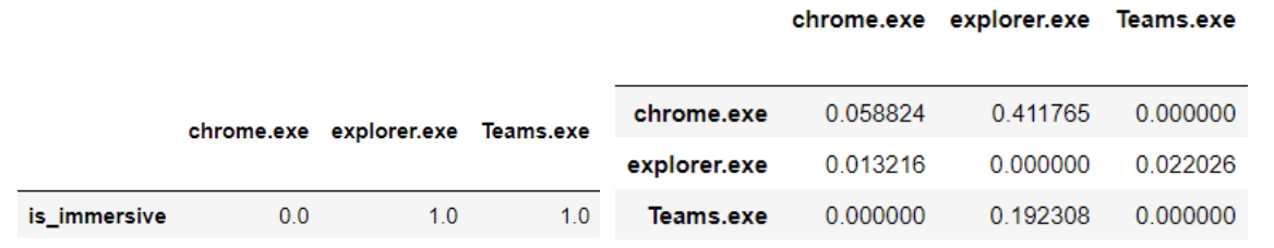
The Hidden Markov Model is a statistical model that we used to predict an app launch based on the sequence of prior app launches. This model uses a Markov Chain, a sequence of possible events in which the probability of each event depends only on the state attained in the previous event. In our case, we will be basing the conditional probabilities on the sequence of possible apps. We utilized data from foreground_window.IL which produced window data as well as is_immersive data, all with timestamps. Since there were no apps that were unresponsive, the is_hung column was dropped. We did not delete the duplicates as it was important to see if an app would be opened after closing that same app. Feature engineering for the HMM involves the construction of transition and emission matrices. The transition matrix is an n x n matrix where n is the number of unique windows. The values in this matrix are the conditional probabilities of switching from one app window to the other. The emission matrix is a 1 x n matrix where n is the number of unique windows and the values contain a feature of each window. In our case, that feature is whether the window is immersive (belongs to the windows app store). This matrix allows us to enhance the accuracy of our model. The HMM can then be visualized as a as seen below:

We proceeded to build 3 predictors for our HMM.

Predictor 1

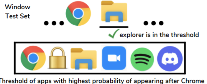
For each test window in the series, the first predictor lists the top 6 (threshold value) most probable windows from the transition matrix. If the next test window is one of these 6 predicted windows, it is assumed to be a correct prediction. A tally of correct and incorrect predictions is maintained at each iteration and an accuracy percentage is outputted based on the final tally.

Predictor 2

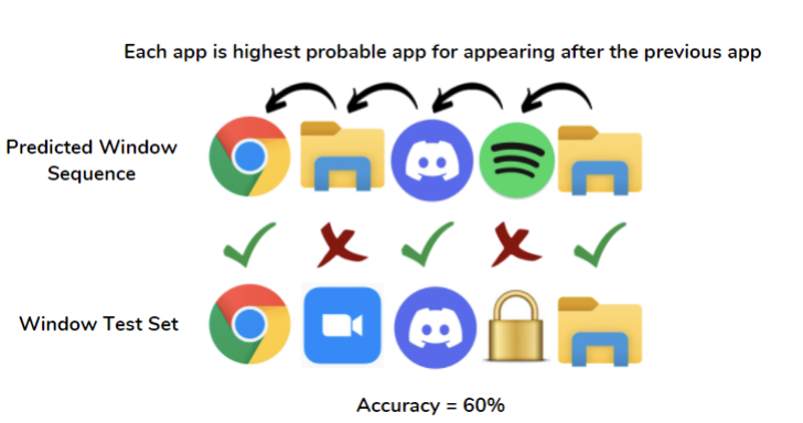
On the other hand, the second predictor returns a sequence of predicted windows. Starting from the first test window, this predictor predicts the next window to be that with the highest probability in the transition matrix. This process is continued iteratively for each test window, and a sequence of windows is then returned. The test accuracy is measured by comparing the predicted sequence output to the test sequence of windows.

Predictor 3

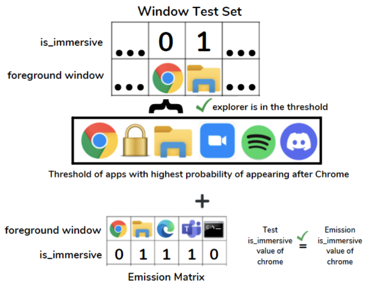
The third predictor is the same as the first with one exception. It uses the emission matrix as well as the transition matrix to assess correct matches. This means that the predicted is_immersive value must also match the test is_immersive value. If either of the conditions are not met, the incorrect tally is incremented in the accuracy calculation. We intend to include more observed variables from desktop mapper outputs in coming weeks which will increase the number of rows of the emission matrix. Although doing this will increase the conditions for a window to “pass”, the test accuracy will be validated further.

HMM Results

Since we had three predictors for the HMM, we ran all of them on the data and yielded the accuracy table presented below:

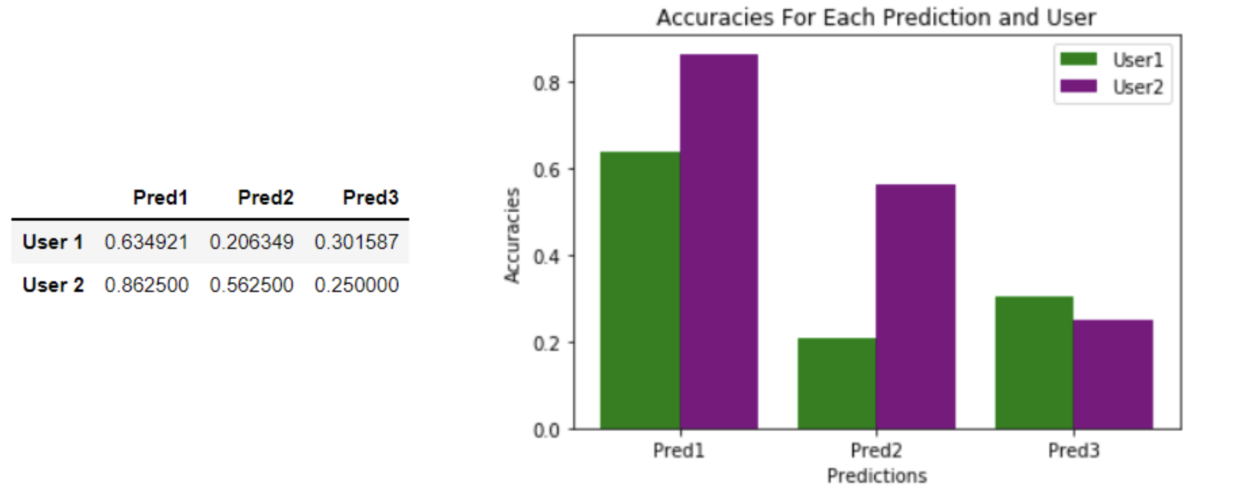
While the HMM was a good model to use in this scenario, there are drawbacks to using one. For example, the seasonality of the data is missing in the transition matrix representation. Because this is a first order HMM, it depends only on the previous application. The large size of the transition matrix for data collection periods of several weeks makes feature engineering a relatively time and memory expensive model to use.

Prediction Problem 2

Univariate Regression

Our first implementation of the LSTM model forecasts the time spent on a certain app by the hour. The architecture of this solution consists of a stacked LSTM model which helps with adding a level of abstraction to input observations over time. The model is trained on a single feature for each app denoting the time spent across the period of data collection. Preprocessing steps include removing duplicates and anomalies by using a 3 sigma approach verified by an LSTM Reconstruction Loss anomaly detection approach. Hyperparameter tuning was performed using GridSearch where we used all available loss functions, various values for the number of layers/nodes. We have explored results generated by using data from different users as well as time periods.

Regression Results

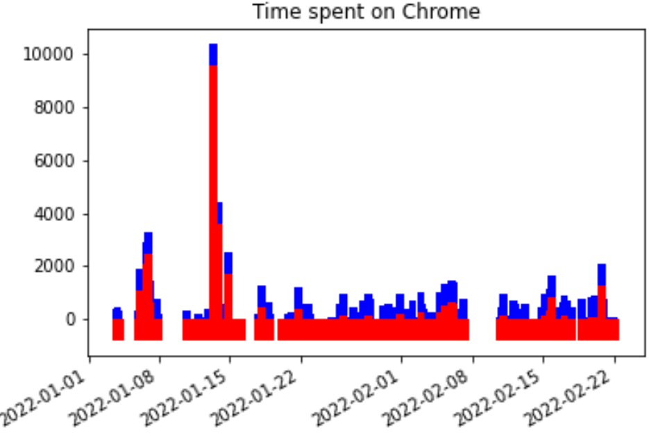
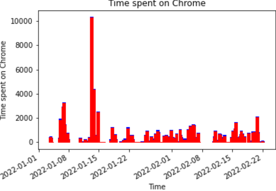
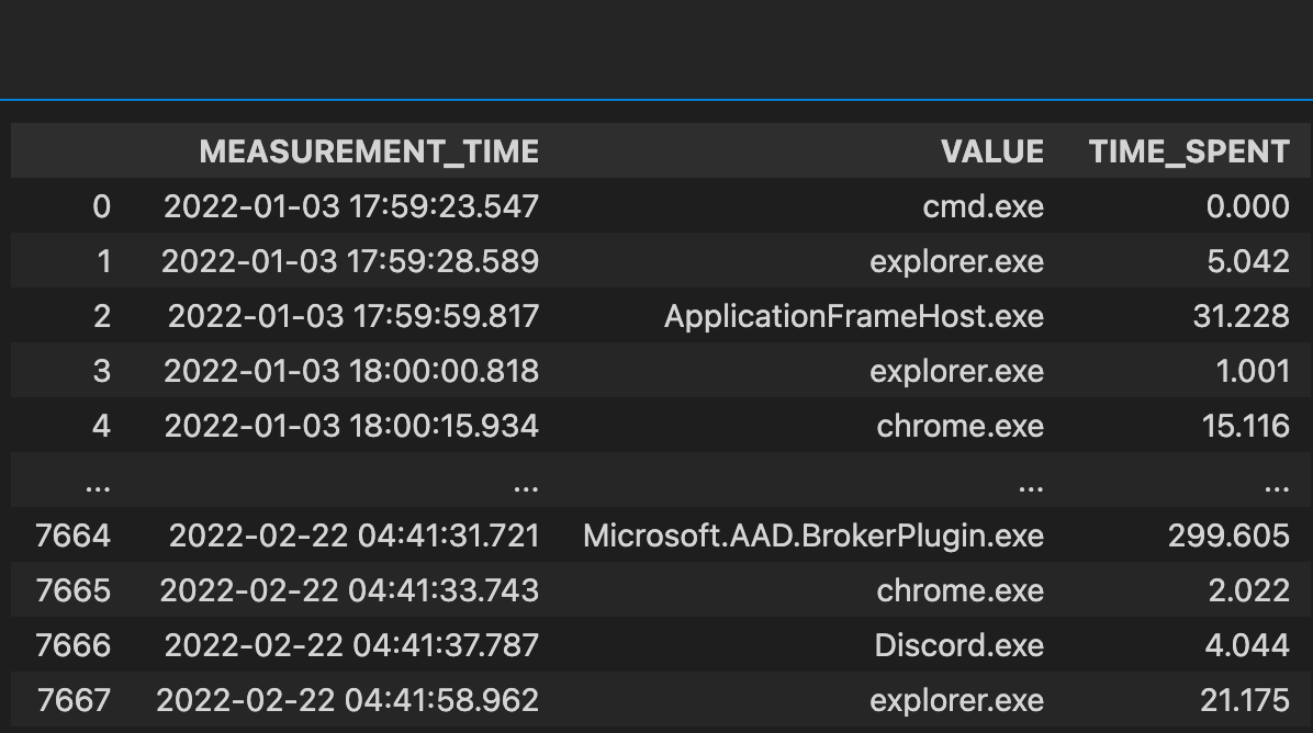
The Stacked LSTM model forecasts the amount of time spent per hour on a particular app. TIME_SPENT values corresponding to the particular app are aggregated to be split into train and test sets. The reported accuracy for TIME_SPENT predictions on training and testing sets are combined for the top 10 apps below. The discrepancy in accuracy values can be attributed to the differences in app usage in each dataset with there being 32 distinct apps for User1 and 25 distinct apps for User2. The accuracy is set to a precision of +/- 10 seconds.

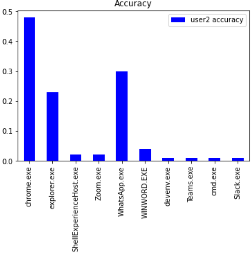
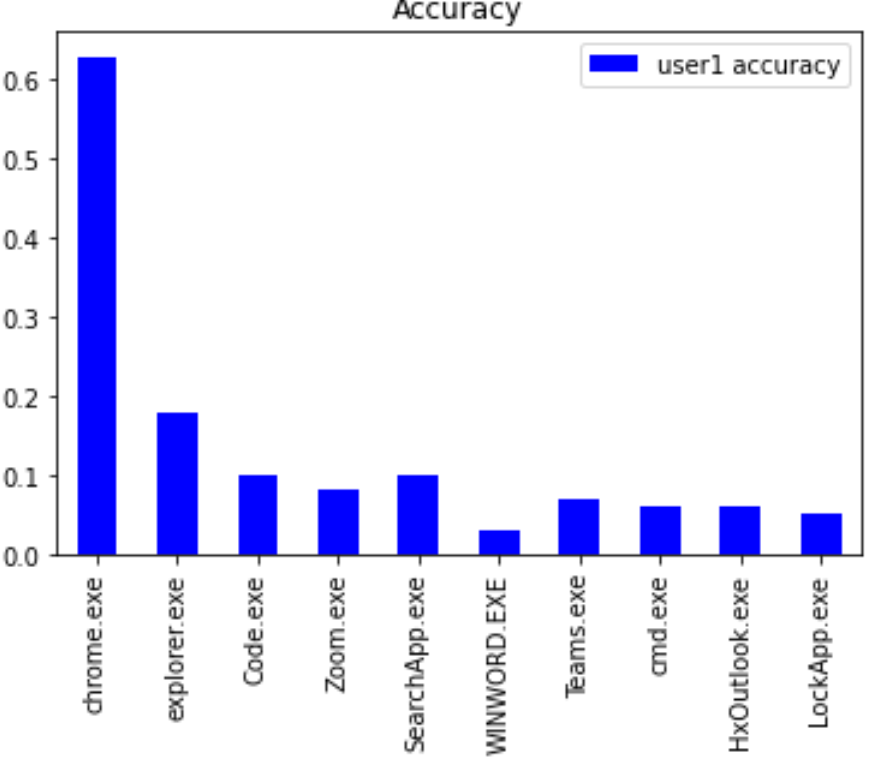
Since the predictions on Chrome were better than that of a coin toss, we will focus on forecasting results for Chrome data. Performance for other apps did not cross this threshold. Due to the significantly low usage of other apps compared to Chrome by both users, the data points were not sufficient to make a reasonable estimate of usage time. The red bars in the figures above represent the prediction values while the blue bars indicate the training and testing data.

The second problem is to predict app usage durations and corresponding app sequences.

The LSTM is appropriate for our second solution since it’s typically used for forecasting problems without being affected by the vanishing gradient problem where convergence happens too quickly. For the second prediction task, we attempted two approaches to the problem: a univariate regression and a multivariate classification.

LSTM Model

The Long-short term memory model, otherwise known as the LSTM, is a recurrent neural network that is well suited for time-series forecasting and sequence prediction problems. The LSTM is structured on memory blocks that are connected through layers. It uses backpropagation of layers and time-step lookback values for model training. Before we trained the model, we performed data cleaning on our datasets for two users. Since we had sporadic occurrences of duplicate windows occurring when apps were in split screen or were resized, we dropped consecutive duplicates since the two windows account for the same app executable. We also removed anomalous executables that appeared only once and never again such as app installers or random popups. The remaining cleaning steps are enumerated below:

1. Convert ‘time’ from string to datetime
2. Calculate time difference between each row
3. Drop unnecessary columns ('ID_INPUT', 'PRIVATE_DATA')
4. Select 3 week time frame
5. Remove windows appearing only once
6. Drop NULL values

Multivariate Classification

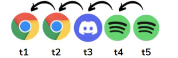
We came up with the second classification approach which predicts app sequences. But since we made the decision to log foreground window data at irregular time intervals, determining the timestamps associated with our predictions was tricky. We made the logging decision to suit the regression approach at the time, so overcoming this problem for classification required us to transform our data to regular time-steps. This was done iteratively such that if there were no windows in the target time-step, we appended NaN. If there was only one window in the time-step, it was appended. If there were multiple windows opened during a particular time-interval, we logged the window that the user spent the most time on during that time interval. A data frame was then tabulated, and the NaNs were forward-filled to account for missing values. In the data shown below, the target time-step is 1 minute.

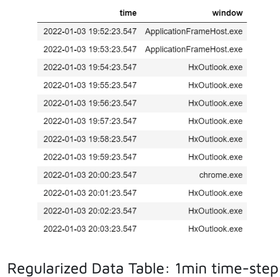
This results in a slight loss of accuracy to the original data, but since our selected time intervals are so small, that loss turned out to be negligible. To have zero loss in regularization, we would actually have to go back and change the foreground window input library to log data at definite time intervals. However, we only came up with this custom approach in the second half of the quarter so we couldn’t collect an additional 3 weeks of data on our PCs. Next, we had to transform the data so it would be accepted by the LSTM for classification. We label-encoded and one-hot encoded our window strings before the data was split into training (60%), testing (20%), and validation (20%) sets, each of which had to be engineered for a supervised learning problem. This is where we tested different look_back values which dictate how many previous sequence elements to use to predict another sequence. When the look_back is 3, a sequence [1,2,3] may predict [4,5,6]. The next training example [2,3,4] predicts [5,6,7] and so on. For our model, a sequence of one-hot vectors was used to predict another sequence of one-hot vectors in this fashion. The predictions were then decoded to give us back the predicted app executable name labels. The model itself was a Keras Sequential model. It has one LSTM layer that returns sequences and an activation layer using softmax activation for multiclass prediction. The model was compiled using the categorical_crossentropy loss and categorical_accuracy as the evaluation metric. We chose the time_interval, look_back, number of nodes, and batch_size for hyper-parameter tuning, resulting in 81 different models trained separately for each user’s data. We tested the following hyper-parameters:

• time intervals = [10s, 30s, 1min]
• look_back values = [3, 6, 12]
• node values = [16, 32, 64]
• batch_size values = [6, 12, 24]

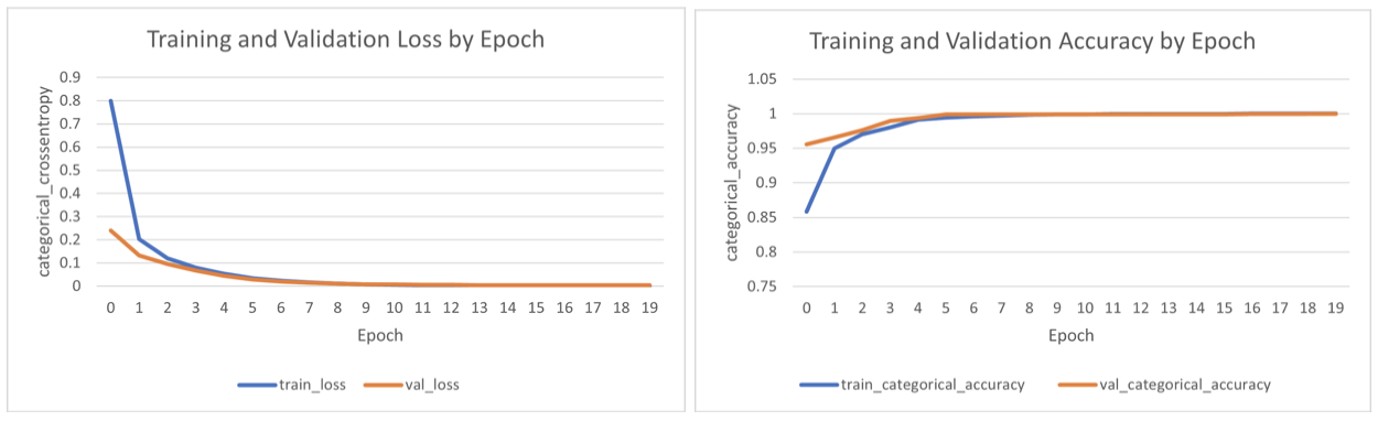
We trained our models for 10 epochs as we found it to be optimal from the training, validation loss and accuracy curves. 10 epochs is the point where the validation loss became smaller than the training loss. To prevent overfitting, we should not run the model for further epochs.

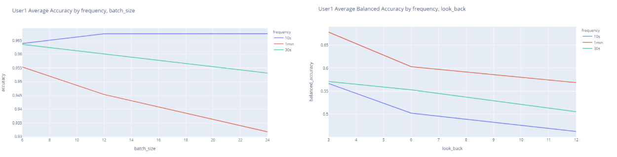
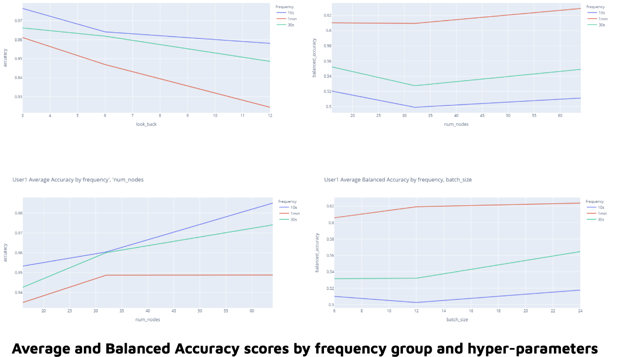
Here we see how each parameter affected model accuracy and balanced accuracy scores for each frequency group. First we note that the 10s frequency group outperforms all others when it comes to accuracy scores while the 1min frequency group does the same for balanced accuracy scores. Next, we observe that a smaller look_back and batch_size give us higher accuracy scores. More nodes also give us higher accuracy scores. The same is true for balanced accuracy scores with the exception of batch_size, which does the opposite. We were accordingly able to deduce the best parameters for our model. We wrote code to test all 81 hyper-parameter combinations for both user’s data. This code programmatically saves each model’s artifacts and training logs to a csv file, as well as the output accuracy scores by parameter combination. Additionally, the code programmatically saves plots describing app usage behavior for each user overlaid by model predictions. These results can be seen in the following section.

LSTM Results

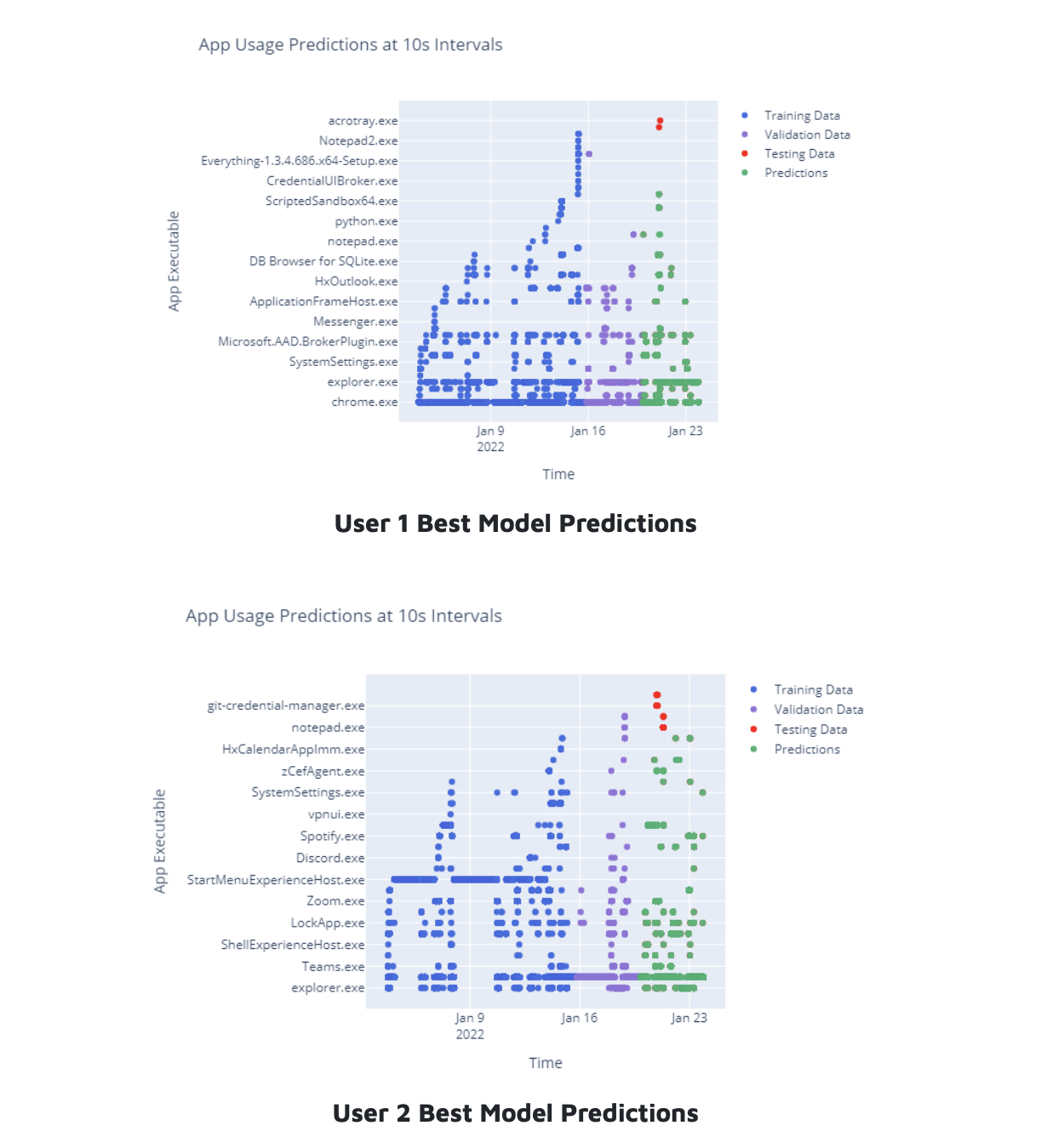
These graphs summarize app usage behavior for both users. On the x-axis we have the data collection time period of 3 weeks over 10s intervals. On the y-axis, we have the app executable used at each time-step. Each dot therefore represents the app used in a particular 10s interval. Here you can see the entire dataset split by training, validation, and testing sets, which is then overlaid by our best predictions for each user. You can see the effectiveness of our approach by looking at the green prediction dots which almost completely overlay the red testing dots. We evaluated our models using several evaluation criteria: the accuracy, balanced_accuracy, weighted f1 score, weighted precision, and weighted recall. We limit our discussion to the accuracy and balanced accuracy scores for this report. The accuracy score is straightforward: of all the predicted windows, what percentage matched the unseen test windows? The balanced accuracy makes a different assumption. It assumes that each class label is equally important. It calculates the prediction accuracy for each individual app, and averages them to give one score. Since our data was heavily imbalanced, we figured both these scores would provide context for our results.

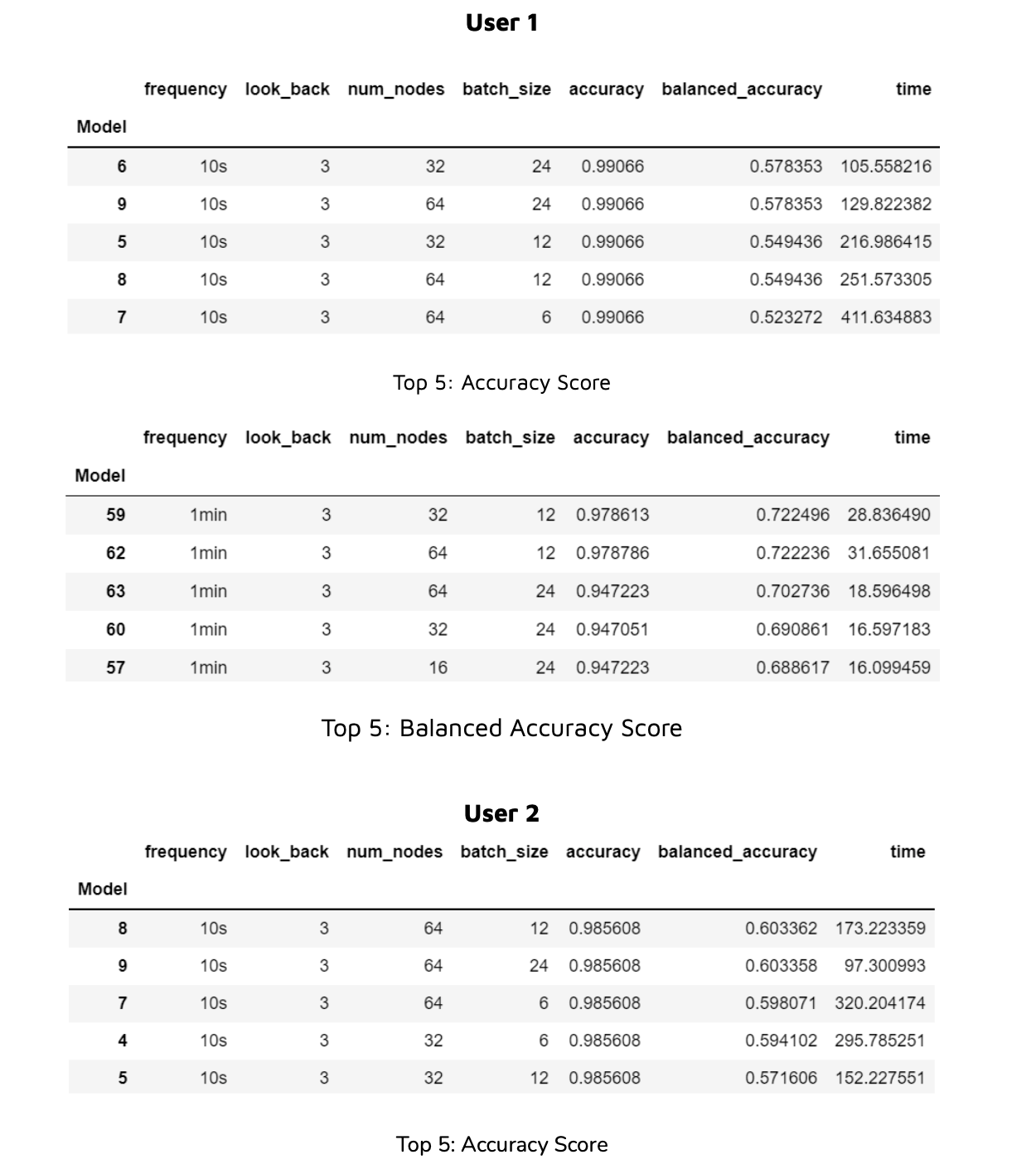
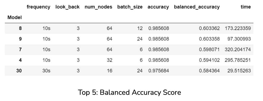
We achieved a stunning accuracy score of 99% for User 1 and 98.5% for User 2. We achieved a more moderate 72% balanced accuracy for User 1 and 60% for User 2. This may be because User 2 had higher relative chrome usage resulting in more imbalanced data.

Conclusion

For the past 20 weeks we have developed various data collectors modules like mouse input, foreground window, user wait, and desktop mapper to collect data for our specific use case. Using the collected data, we built predictive models using autoencoders like LSTM and generative models such as Hidden Markov Models. The high accuracy of our predictive models imply that they can be used to effectively infer the sequences of apps used on a daily basis and how long each app is used. The design decisions made during the process which include using the memory management capabilities of C for the data collectors and using RNNs for our predictions were mainly for scalability and future expansion goals.

Real-World Implications

The implications of our multivariate LSTM results are massive. Successfully forecasting app usage behavior means that we can further optimize the PC experience. Knowing when an app will be launched by the user means we can launch it preemptively in the background and largely eliminate that dreaded spinning wait cursor. And knowing how long apps will run would allow us to optimize system resources such as battery and memory. This solution can be very beneficial especially on low spec Windows machines which cannot have daily used apps constantly open in the background.

Future Plans

A typical data scientist rarely has control over the data collection process as the task is delegated to software engineers who build tools from which data is extracted. Since we built our own collector modules we were able to define the exact inputs needed for our model, control the polling frequency of the data, and define custom wait signals for data collection. We plan on modifying our existing foreground window collector to log results at regular time-series instead of mouse click burst events to eliminate lossy regularization. We also want to tune our desktop mapper collector to provide more reliable results. This way, we can enhance our multivariate LSTM and add new features to the emission matrix for HMM.

However, to really earn the label of all star data scientists, we must also take upon the role of an ml engineer by paying attention to potential privacy concerns. We wish to:

• Generate a unique hash for each users data.
• Come up with a cloud based analytics system would stream data to AWS S3 and use other AWS resources like EMR and Sagemaker to run and deploy training jobs.